Simulated data for GAM's

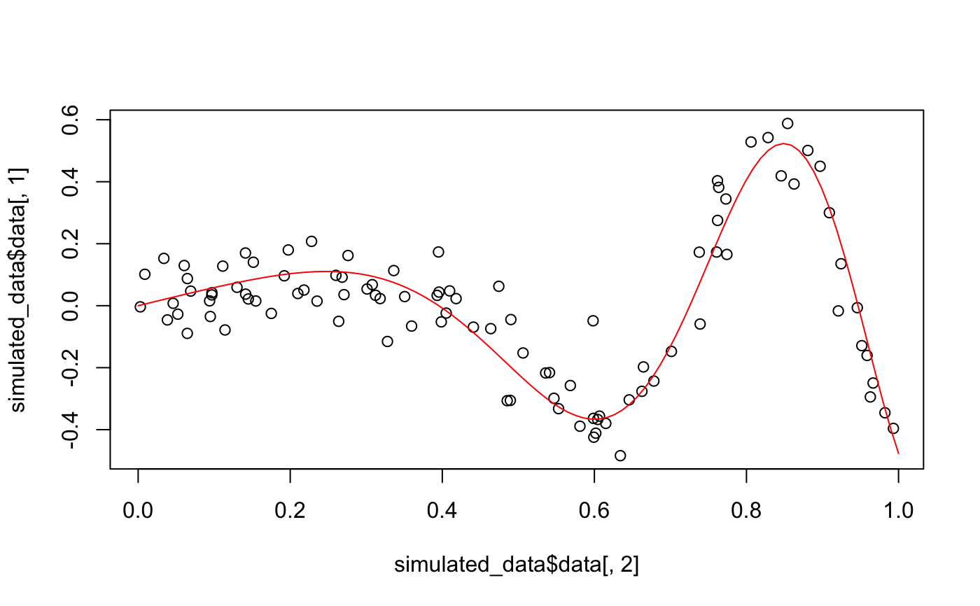
This function creates simulated datasets to illustrate the use of gam3.

gamSim2(n, p, test.n, sigma, probs)

Arguments

n	numeric value specifying the number of observations.
p	numeric value specifying the number of covariates.
test.n	numeric value specifying the number of observations in the test set.
sigma	numeric value specifying the standard deviation of the errors.
probs	numeric vector of length 6 specifying the proportion of covariates that are polynomial, linear, exponential, logarithmic, sinusoidal, and zero functions.

Value

A named list containing data, functions, line, and test.

data

An n\(\times\) p+1 dataframe containing the simulated data. The first column contains the response, with all subsequent columns containing the covariates.

functions

A list of length p containing the true functions.

line

A character vector of length p containing the type of function used.

test

An test.n\(\times\) p+1 dataframe containing the simulated test data. The first column contains the response, with all subsequent columns containing the covariates.

Details

This function creates simulated datasets to illustrate the use of gam3. The covariates are sampled uniformly over $[0, 1]$, and their associated functions are randomly chosen from polynomial, linear, exponential, logarithmic, sinusoidal, and zero using weights provided in the probs argument.

Examples

set.seed(2018)
probs <- c(0.1, 0.1, 0.1, 0.1, 0.1, 0.5)
simulated_data <- gamSim2(n = 100, p = 1, test.n = 20, sigma = 0.1, probs = probs)
# -1*2*x*sin(2.70259540737607*pi * x^2 - 1.3270146084221)
sin.fun <- function(x) eval(parse(text = simulated_data$functions[[1]]))
truth <- sin.fun(seq(0, 1, length.out = 100))
truth <- truth/diff(range(truth))
plot(simulated_data$data[, 2], simulated_data$data[, 1])
lines(seq(0, 1, length.out = 100), truth, col = "red")